Surface Facilities

Facilities include any of the elements (e.g., delivery points, compressors, wells, etc.) that you can add to the GIS map.

Delivery Points

A Delivery Point in Piper is considered to be a gas destination of sufficiently constant pressure that it can be considered to not vary as a function of gas rate. A Delivery Point is configurable on date basis, so it can vary from one date to the next. The only attribute of a Delivery Point is its Delivery Pressure.

There must be at least one delivery point in a model for the model to converge. More than one delivery point is allowed.

Multiple Delivery Points and Loop Links

There are many instances or reasons why the user may choose to incorporate multiple delivery points into a single Piper model.

In one case, the user has two separate systems and each system is delivering to separate locations. They may want to build the two systems in a single Piper file because at some point in the future a linkage between the systems may be built. Here, the two separate gathering systems can be constructed in a single file and no loop link needs to be defined. Once connectivity between the multiple systems within a single Piper file is made, a loop link needs to be defined. Loop links can be selected within the software in one of two ways.

In a second case, the user may have a single gathering system that can deliver to two separate plants. They would like to model both plants and see how the gas is distributed between delivery points. Depending on the default settings (e.g., the default loop link selection method, which can be accessed from the default dialog box), you must select a loop link, or choose to have the software select a loop link based on an internal set of looping rules.

The forecast routine that Piper uses to solve files that contain multiple delivery points creates a pseudo flow loop within the system. When a flow loop is created in a Piper file, a loop link must be defined. Defining a line in a flow loop as a loop link is used within the software’s forecast routine and allows for the desired system flows and pressures to be calculated.

In systems where the user has defined more than one delivery, Piper defines a “primary” or “hidden” delivery point. This Primary Delivery Point is an internal point, visible to the software only. All user defined delivery points are linked to this internal point. The following images illustrate the difference between what Piper displays on-screen (to the user) and what the software “sees” internally.

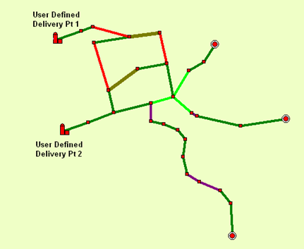
When the defining two delivery points within a single Piper file, the user sees the two delivery points that have been added either by on-screen techniques or through the delivery point editor. The loop links within the system can be distinguished by the yellow/green line color ( ).

The following image shows what is used internally within the software; it represents what is used in the software forecasting routine. Piper sees a Primary Delivery point through which all system gas must flow, and two single suction compressors that are attached to the Primary Delivery with null diameter lines of 1 mile length. Each additional delivery point defined in a multiple delivery point model will be represented internally in the same manner and connected to the Primary Delivery as stated above.

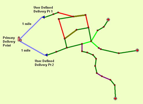
Note: When multiple delivery points are defined in Piper a flow loop has been created and a loop link needs to be defined.

Two methods exist for defining loop links within the software:

1. User Defined Loop Links (user selects the location of loop links and designates the chosen link as a loop link)

2. Piper automatic loop link selection (software selects the loop link based on a set of pre-defined looping rules contained within the software)

For additional information on loop links, see adding loop links.

Expected behavior when multiple delivery points are added

Multiple Delivery Points in a Single Connected Gathering System

When multiple delivery points are connected to a single gathering system, and the auto-loop link routine is enabled (the default for new models), the user should expect that the Piper will define an additional loop link in the system that represents the connection through the two delivery points. For each additional delivery point, users should expect an additional loop link.

When multiple delivery points are connected to a single gathering system and if the auto-loop link routine is not enabled (the default for an existing model built in a previous version), the user will have to define a loop link that will represent the connection through the two delivery points. The steps for doing so are provided below, but for beginning users not familiar with loop links it is advised that you contact IHS support for help.

1. When the second (third, fourth, etc) delivery point is added and connected to the, a notification will be provided in the status window that a loop has been added and a link disabled.

2. Make note of the link that has been disabled.

3. Go into the Gathering System editor and find the link that has been disabled.

4. Re-enable the link and define it as a loop link by toggling on the “Looped” toggle and giving the link a UID

5. Exit the Gathering System editor

6. Press Ctrl-L and hover over the loop link that was just added to view the loop – note the loop that should go through the two delivery points

7. If the loop link is not in an ideal location (as per the rules of looping), modify the loop link as needed

Multiple Delivery Points in Unconnected Gathering Systems

When multiple delivery points are added to unconnected gathering systems, the user should expect that no loop links will be added by Piper. The systems should behave independently. It is only internally during the solution process that Piper will treat the delivery points separately

Loops

Rules for Line Looping

These are the current "rules" for using the line looping in Piper. Loop links are designated in the gathering system editor by mouse clicking the toggle in the "Looped" column for the appropriate link.

1. Only one loop link can be designated for each loop; otherwise, Piper will not be able to complete the connection and a "Link not used" error will occur. The second loop link is not valid.

2. Two loops can not share the same loop link.

3. In flow loops, a loop link should be located near nodes where gas flow is expected to split. That is, where the flow direction "arrows" diverge as opposed to where "arrows" converge. A quick way to do this is to place the loop link in the loop as far away from the delivery point as possible. Another preliminary way to do this is to place the loop link at a point in the loop that is equidistant in each branch from the delivery point. Start by counting the number of links in each branch required to reach the proposed loop link.

4. Do not connect loop links to the delivery point, compressors, contracts, dehydrators or refrigeration facilities. The only valid nodes for connecting loop links are nodes with no attached facilities and nodes with wells. Do not designate links with any other node type as loop links. Piper may not always transfer gas and liquid volumes accurately in these situations.

5. Compressors, contracts, dehydrators and refrigeration facilities should generally be located between the delivery point and loop links. This pre-supposes that the loop link has been placed at a point in compliance with point # 3. These facilities orient themselves such that their inlets face the loop link and their outlets face the delivery point. Note in the following schematics the loop link should not be connected to the delivery point, compressors, contracts, refrigeration facilities and dehydrators.

Unique ID

The unique ID is used as an internal identifier by Piper. The user must specify the unique ID for each loop that is specified. The unique ID can contain either a letter or number designation. It is only required that no two unique ID's use the same identifier.

Displaying or Hiding Loop Links and Loops

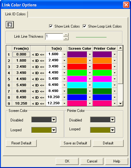
The loop links chosen either by the user or by Piper will, by default, be displayed on-screen with a thick, gold colored link. Loop links can be hidden from display through an option in the Link Colors Options to “Show Loop Link Colors”.

To display the loop that a loop link is associated with, the Ctrl-L command can be used. After pressing Ctrl-L, with the mouse cursor, hover over the loop link that is of interest. The loop that the loop link is associated with should become highlighted in two colors, orange and blue. The two colors represent the two potential directions of flow around the loop. Where the blue and orange line converge and form a single orange line, that is where the loop ties back into a single line. See the figure below for an illustration:

Tips

Before constructing a complicated gathering system that includes flow loops, create a simplified sketch of the system and identify ALL loops. Then, choose the line loop locations based on the above rules.
Since Loop Links are special links that are really termination points for connected branches, it is possible to specify loop links that isolate links from the delivery point. Piper will interpret isolated links as unused facilities and disable those links. Disabled links and facilities will not be displayed on-screen.

If a portion of a gathering system is not shown on-screen and a list of  "Link not used" errors is displayed in the status window, DO NOT PANIC. This message indicates a link node name may have been improperly entered or the designated loop link violates one or more of the above rules. Review the above rules and designate a different link as the loop link to solve the problem.

Nodes

Nodes are connection points. Each Link in a gathering system requires a Source Node name and a Destination Node name. Separate links each having the same node names will be connected together. Successive links, joined by the ends having identical node names, form the gathering system model we see on-screen. The Source node name and Destination node name cannot be identical for a single link.

Nodes are displayed on-screen as squares to make it easier to see and work with them.

Nodes allow the attachment of various facilities such as wells, compressors, contracts, dehydrators, NGL recovery units (Refrigeration) or amine plants. Only one facility can be attached to a node at one time. This was done to simplify display options as it eliminates the need for combination symbols or setting up a hierarchy of symbols used to represent each of these facilities.

Source Node

The Source Node Name is the name given to the source node for each Link in a gathering system model. This can be any alphanumeric combination; for example Junction 23-4, or well 3-16-24-32 W4M, or Watering Hole. For your convenience, the program does not differentiate between uppercase and lowercase letters. For example, B-34 is equivalent to b-34. Use of spaces, alphanumeric and numeric characters as well as other symbols such as dashes (-), underscores (_), plus signs (+), number signs (#), slashes (/), etc. are allowed.

UNITS: None

DEFAULT: None

Destination Node

The Destination Node is the name given to the Destination for each Link in a gathering system model. This can be any alphanumeric combination: for example Junction 23-4, or well 3-16-24-32 W4M, or Watering Hole. For your convenience, the program does not differentiate between uppercase and lowercase letters. For example, B-34 is equivalent to b-34. Use of spaces, alphanumeric and numeric characters as well as other symbols such as dashes (-), underscores (_), plus signs (+), number signs (#), slashes (/), etc. are allowed.

UNITS: None

DEFAULT: None

Node Gas Rate

This is the measured gas rate through a particular node in the gathering system. This information along with the Measured Pressure can be displayed on screen and used to tune the model.

UNITS: MMscfd (103m3/d)

DEFAULT: None

Node Liquid Rate

This is the measured liquid rate at a node in the gathering system.

UNITS: bbl/d (m3/d)

DEFAULT: 0

Node Measured Pressure

This is the measured pressure at a particular node in the gathering system. You can access the Measured Pressure from the Node editor. This information can be displayed on screen and used to tune the model.

UNITS: psia (kPaa)

DEFAULT: 0

Node Remarks

This field allows for the entry of Node specific remarks. The user can display these on the gathering system map.

UNITS: None

DEFAULT: None

Compressors

There are primarily two types of compressors used by the petroleum industry. These are reciprocating compressors and rotary screw compressors. The Piper approach to modeling compressors is independent of the compressor being modeled, so the user should be able to model both compressor types. The user is expected to supply information that should be readily available from the manufacturer. The user is encouraged to always plot current conditions of suction pressure and throughput to ensure that the compressor is being utilized at or near to design specifications.

It has been our experience that operators rarely utilize compressors at design specifications. Some common reasons that the actual utilization differs when compared to design are as follows:

• reduced RPM's
• unloaded head-end in double acting compressors
• utilization of valve pockets to reduce capacity
• multiple units
• modification to basic clearance volumes

Physical Description

The unit we commonly call a compressor is really two separate machines that have been joined together. The driver is an engine that supplies the energy or horsepower to compress the gas.

The design of a compressor is a complex task as it must account for the compression of a non-ideal gas with its associated thermodynamic properties and the mechanical requirements of the machinery which has limits for volumetric efficiency, mechanical loads, temperature restriction and operating pressure restrictions.

Modeling Compression

In general, there are three ways of handling Compressors in Piper:

1. No Compressor Curves or Horsepower Limitations specified: this option is generally used when attempting to get a preliminary idea of deliverability and horsepower requirements. This method estimates the horsepower required to maintain the specified Minimum Inlet Pressure. Since this method will maximize deliverability without regard for the realities of compressor sizing, it should only be used to determine peak horsepower requirements. This approach to compression is generally used in model calibration, where only the current condition of operation of the compressor is desired. This approach can also be used to model secondary compression, as the primary compression will dictate the secondary compressors performance.

2. No Compressor Curves but Horsepower Limitations apply: we call this the infinitely flexible Compressor as it assumes the compressor will be physically configured, as required, to handle whatever gas rate the field can supply at a given Inlet Pressure and maximum available horsepower. This method is used mainly to generate deliverability forecasts for a range of horsepower limitations to provide an accurate estimate of long-term deliverability versus installed horsepower. This method assumes the operator will reconfigure the Compressor as required to maintain optimum deliverability within the bounds of the specified Minimum Inlet Pressure and maximum Horsepower Available.

3. Specify Compressor Curves: this option accurately calculates the relationship between Compressor Capacity and field deliverability. Compressor Curves are generally available from the manufacturer. However, if they are not available and the Compressor is currently working at its capacity, input the current measured suction pressure and gas throughput in the Maximum Inlet Pressure and Maximum Inlet Rate columns, respectively. Ensure the measured discharge pressure for the compressor is reflected in the model match. This methodology will provide an accurate compressor curve for the current compressor configuration. This method can be very pessimistic when used for long term deliverability forecasting as the compressor may have other configurations that have not been used yet.

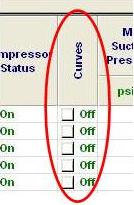
To turn the capacity curves function on, click the "Curves On/Off" toggle situated under the Compressor type column, in the Compressor Editor. Piper will open the cells corresponding to the Maximum Inlet Pressure, Minimum Inlet Rate, Maximum Inlet Rate, Minimum Inlet Pressure, Mid Inlet Pressure and Mid Inlet Rate for data input.

Compressors using Capacity Curves

This option uses compressor capacity curves to simulate the compressor performance. Compressor capacity curves define a specific compressor configuration. In Piper, a specific compressor configuration means the current valve pocket settings, number of stages, etc.

The program uses this information to internally construct a straight line Suction Pressure versus Inlet Gas Capacity correlation for the compressor. These variables can be scheduled through time making modeling of various compressor configurations relatively easy.

Compressor curves are generally presented by the manufacturer as follows:

The lower curve represents the relationship between suction pressure and gas rate. The simplest version of this relationship is a straight line passing through the origin.

Gas Rate = Slope x Suction Pressure

which is defined in the program by input of the Maximum Inlet Pressure and Maximum Inlet Rate. By using this methodology the program can completely define the compressor curve with three (3) input variables. These parameters define the upper limit of a compressor's range. The lower limit of the range is defined by the Minimum Inlet Pressure .

The Figure shown below demonstrates how the program calculates the compressor inlet pressure and gas throughput called the operating point. The deliverability available from the field is shown as a downward sloped curve, whereas the compressor curve is an upward sloped straight line. The intersection of these curves is the operating point.

In the situation where the field has more deliverability than the compressor can handle, as shown in the Figure below, the program invokes a choke between the Inlet and the suction of the compressor. This drops the pressure the compressor sees to its Maximum Inlet Pressure.

In the situation where the field does not have sufficient deliverability at the Minimum Inlet Pressure for the compressor to properly fill the cylinders, the compressor will invoke a recycle stream to maintain the required volume of gas as dictated by the compressor curve. The compressor will consequently continue to produce at its Minimum Inlet Pressure and corresponding minimum gas rate while the net gas rate discharged by the compressor will be equal to field production. The lowest limit for this scenario occurs when the field can no longer supply gas at the Minimum Inlet Pressure of the compressor. At this point the compressor will be on 100% recycle.

Compressor Curves are generally available from the manufacturer. However, if they are not available and the Compressor is currently working at its capacity, input the current measured suction pressure and gas throughput in the Maximum Inlet Pressure and Maximum Inlet Rate, respectively. Ensure the measured discharge pressure for the compressor is reflected in the model match. This methodology will provide an accurate compressor curve for the current compressor configuration. This method can be very pessimistic when used for long term deliverability forecasting as the compressor may have other configurations that have not been used yet.

On-Stream Date

The date in which a compressor is to become active in the forecast interval set in the Forecast View tab. A compressor becomes active on the later of the on-stream date or the first date of the forecast interval. If the on-stream date is blank, a compressor is active the first forecast date.

UNITS: MM/DD/YYYY

DEFAULT: None

Minimum Inlet Rate

The Minimum Inlet Rate, Maximum Inlet Pressure and the Maximum Inlet Rate input cells become active in the compressor editor when the Compressor Curves function is turned on. The Minimum Inlet Rate defines the lower gas rate capacity for a specific compressor. The Minimum Inlet Rate should be obtained from compressor manufacturer performance curves. If not specified, the minimum inlet rate will be calculated based on the assumption that the capacity curve will be a straight line going from "0" capacity and "0" pressure to the input data for maximum inlet pressure and maximum inlet rate.

UNITS: MMscfd (103m3/d)

DEFAULT: 0

Mid Inlet Rate

The Mid Inlet Rate input cell becomes active in the compressor editor when the Compressor Curves function is turned on. The Maximum Inlet Rate defines the upper gas rate capacity for a specific compressor. The Maximum Inlet Rate should be obtained from the compressor manufacturer performance curves.

UNITS: MMscfd (103m3/d)

DEFAULT: None

Maximum Inlet Rate

The Minimum Inlet Rate, Mid Inlet Rate, Mid Suction Pressure, Maximum Inlet Pressure and the Maximum Inlet Rate input cells become active in the compressor editor when the Compressor Curves function is turned on. The Maximum Inlet Rate defines the upper gas rate capacity for a specific compressor. The Maximum Inlet Rate should be obtained from the compressor manufacturer performance curves.

UNITS: MMscfd (103m3/d)

DEFAULT: None

Minimum Suction Pressure

Minimum Suction Pressure is the lowest achievable suction pressure for a compressor. This value is a function of the compressor design and is determined using the compressor capacity curves.

UNITS: kPaa

DEFAULT: None

Mid Suction Pressure

Mid Suction Pressure is the mid-point achievable suction pressure for a compressor. This value is a function of the compressor design and is determined using the compressor capacity curves.

UNITS: psia (kPaa)

DEFAULT: None

Maximum Suction Pressure

Maximum Suction Pressure is the maximum achievable suction pressure for a compressor. This value is a function of the compressor design and is determined using the compressor capacity curves.

UNITS: psia (kPaa)

DEFAULT: None

Other Compressor Terminology

Horsepower Utilized and Available

The horsepower utilizedis the amount of energy that is required to maintain the specified state of operation of a compressor. Piper calculates horsepower used based on the assumption that the compression process is an isothermal process. Piper then corrects the result by a 10% safety factor. The resultant equation that Piper uses to calculate horsepower is:

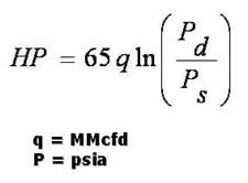
This equation builds the effect of gas gravity, compressibility, inlet temperature as well as the 10% safety factor into the constant of 65. There is no consideration in the calculation for any losses. Only the energy required to compress the gas is considered

This horsepower utilized is always equal to or less than the horsepower available.

The horsepower available in Piper is the maximum horsepower available to compress the gas. The compressor drive motor is generally sized to match the compressor capacity requirements. However, if the Horsepower Available is undersized relative to the compressor capacity and field deliverability, Piper will progressively choke the inlet pressure at the compressor until the utilized horsepower is equal to the horsepower available. This will reduce the gas rate flowing from the field and will create a pressure differential between the inlet and suction of the compressor. Piper differentiates pressure information at the entry to the compressor as the INLET (the backpressure the wells produce against) and SUCTION (the pressure of the gas entering the compressor). If compressor curves are not specified, then Piper will increase the pressure differential until the horsepower limitation is honored. If compressor curves are specified, Piper will again increase the pressure differential until the horsepower limitation is honored but then will also search for a solution that honors the rate capacity - suction pressure relationship defined by the compressor curve. It is extremely important that the horsepower available and the rate capacity - suction pressure relationship be matched sets of data.

Schedule changes in Horsepower Available can be inserted on a monthly basis. The user only has to fill in the months in which a change is made. By clicking the button situated on the right side of each cell, the change will be copied down. Proceed in a similar manner for every change that you want to insert.

UNITS: HP (kW)

DEFAULT: Unlimited

Flow Limit

The Flow Limit option allows you to specify the maximum flow that can go through the compressor. The Flow LImit option allows you to model a valve compressor.

Compressor Fuel Gas

Natural gas compressors consume natural gas as fuel. This gas can be taken from an alternate source or from the gas stream entering the facility. Fuel is taken from the gathering system to run the compressor is called Fuel Gas. The Fuel Gas consumption is related to the horsepower used, which in turn, is related to the volume of gas being compressed. When no horsepower is being used, the Fuel Gas is zero. Fuel usage in Piper is expressed as a percentage of the throughput. A reasonable usage number is 3%. Fuel usage should be entered when tuning a gathering system.

UNITS: Percent (%)

DEFAULT: 0

Pumps

There are two types of pumps modeled in Piper:

• Pump Curve – a curve is required.
• Constant Head – only one operating point needs to be entered.

When entering a curve in the pump curve editor, as the pressure increases, the rate must decrease. Otherwise, an error message will appear.

If the operating conditions fall between or outside of the pump curve, Piper will interpolate along the pump curve points on an iterative basis to determine the pressure change across the pump for a given liquid rate being pumped.

When a constant head is entered, Piper applies the specified head across the pump regardless of the rate being pumped. 

If the rate across the pump is zero, the head applied across the pump is set to zero, as the pump is considered to be off-line.

If the pump converges to an operating point outside of the specified pump curve, Piper will accept the converged solution, but will provide a warning in the status window that the pump may be operating outside of its allowable limits, and in practice, behavior may be unstable.

Efficiency and Horsepower

Piper calculates the pump efficiency and required horsepower using the following equations:

For the range of values:

100-1000 USGPM=4500-45000 bbl/d

Pressure in Head 50-300 ft or 20-250 psi

If the operating conditions fall outside of this range,Piper will calculate the pump efficiency and horsepower, but these values will not be displayed.

Viscosity

For the pump calculations, Piper uses the combined viscosity. The combined viscosity can be displayed at each node and facility and is calculated using the viscosity correlation that has been defined in the Correlations editor.  By default this correlation is Vasquez and Beggs for black oil models, and Lorenz, Bray and Clark for equation of state models.

The viscosity entered in the pump curve dialog box is the viscosity at which the pump curve was created. This means that the associated pressure drop may be different, based on the viscosity difference.

Intakes and Offtakes

Offtakes are used to remove gas from a system at a fixed rate. Offtakes are useful where gas must be delivered at a specific rate and a minimum pressure. Examples would be power plants, fertilizer plants and other industrial or domestic sales points. A typical use of an intake would be cases where gas will be supplied from some third party.

Intakes are used to inject gas into a system at a fixed rate. This means that the model would have to include a source of gas that would not affect the deliverability of the reservoir.

One common use of intakes and offtakes is for the simplification of large gathering systems. A large gathering system may be excessively cumbersome to deal with, and the use of intakes and offtakes to approximate the gas flows in areas of lessor importance can reduce model size and solution time. Another use may be to simulate the existence of multiple gas delivery points.

Stage

This option is only valid for offtakes. By selecting this option, Piper will adjust the rate into the offtake after the minimum pressure of the offtake has been reached. This will continue until the rate reaches zero.

When staging is turned off, gas cannot be delivered below the specified minimum pressure for the offtake.

Minimum Pressure

This option is only valid for offtakes. This is the lowest back pressure against which an offtake is still able to operate. A non-zero entry must be supplied for minimum pressure.

UNITS: psia (kPaA)

DEFAULT: None

Gas Rate

This is the rate of gas that is injected or removed from a system through the offtake or intake. For an offtake with staging active, once the minimum pressure has been reached, this rate will decrease in order to maintain that pressure.

Gas Props

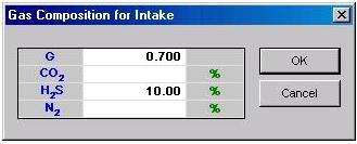
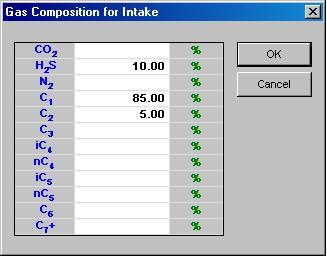
This option is only valid for intakes. This is used to specify the composition of the gas injected that is into the system. The default is use of simplified gas properties (G, CO2, H2S, and N2 only).

If composition tracking is turned on, then the required input switches to a C7+ analysis.

Contracts

Contracts are used to restrict flow through a node to a set value. This value is referred to as the Daily Contract Volume. Contract restrictions are currently calculated based on raw gas throughput at the contract node. Contracts can be located at any available node in the system.

A contract will automatically restrict wells upstream of it to flow at a reduced rate so that the rate through the contract point is not greater then the contracted daily volume. To achieve the desired flow rate, the contract acts as a variable pressure loss, adjusting the pressure loss until it produces the desired contracted volume.

Contracts are represented in the gathering system map as a "Bow Tie".

Contract Status

To access the Contract Status, click on Contracts under the Facilities menu. The Contract Status is a toggle that allows the user the capability to turn a contract on or off regardless of the data entered into the contract editor. Changes to the contract status can be performed throughout the forecast.

UNITS: None

DEFAULT : Off

Daily Contract Volume

To access the daily contract rate, click on Contracts under the Facilities menu. The contract editor window will be open, allowing the daily contract rate input under the daily contract rate column.

The Daily Contract Rate specifies the average daily raw gas rate that can be produced through the contract node. The contract rate is achieved by choking the gas flowing into the contract point.

Changes to the Daily Contract Rate can be done throughout the forecast. For technical and practical reasons, a flow limit input is included with each compressor. This eliminates the problem of placing both, a contract and a compressor at one node.

If you need to give a name to the Compressor Contract (i.e. NVL, TCPL, etc.) this is best done via the Remarks cell. A contract specified at a compressor is assumed to occur at the outlet of the compressor. Compressor Fuel Gas is also removed at the outlet of the compressor but prior to the contract.

UNITS: MMscfd (103m3/d)

DEFAULT: None

Contract Name

Piper treats contracts like a facility that can be attached to a node. To attach a facility to a node, select the appropriate node name from the list of available node names in the contract editor.

UNITS: None

DEFAULT: None

Separators

Separators are used to remove free liquids from the gas stream. Separators can be located at any available node in the system. A fixed pressure loss across the facility and the amount of fuel gas that is to be extracted at this point can also be specified. In Piper a separator can be specified to remove either all or part of the liquids in the gas stream.

Separator Outlet Options

There are multiple options available for the outlet(s) of the separator. These are selected with the drop-down menu in the “Recombine" column. The table below details how outlets are set based on the different options.

Recombine Option	Description
None	Three outlets: gas, oil, and water. Gas is only sent to the gas outlet (there is no gas in the oil or water outlets). The volumes of oil and water removed are sent to their respective outlets with a portion being sent to the other liquid outlet depending on the efficiency of liquid removal from gas and water removal from oil.
All	One outlet with all gas (after fuel gas removed), oil, and water.
Gas Oil	Two outlets: gas + oil and water. The amount of removed water is sent to the water outlet with the remainder sent to the gas + oil outlet. The Oil-Water Efficiency determines the amount of oil sent to the water outlet.
Gas Water	Two outlets: gas + water and oil. The amount of removed oil is sent to the oil outlet with the remainder sent to the gas + water outlet. The Oil-Water Efficiency determines the amount of water sent to the oil outlet.
Liquid	Two outlets: gas and liquid. Only the Gas-Liquid Efficiency is used in separating the volumes of oil and water between the two outlets.

Separator Gas-Liquid Efficiency

Separators typically remove a percentage of the total liquids flowing through them. The amount of oil and water removed from the gas stream is specified as a percentage of throughput.

UNITS: Percent (%)

DEFAULT: 100.00%

Separator Oil-Water Efficiency

When oil and water are primarily sent to different outlets (recombine state set to “None?, “Gas Oil? or “Gas Water?), the amount of oil sent to the oil outlet is the specified percentage of the total removed oil volume from the gas outlet. The amount of water sent to the water outlet is the specified percentage of the total removed water volume from the gas outlet. The remainder of these is sent to the other liquid outlet.

UNITS: Percent (%)

DEFAULT: 100.00%

Separator Fuel Gas

Fuel gas is sometimes required to run a separator. If the facility requires natural gas as fuel and it is taken from the gas stream, this variable will let the facility remove a percentage of the unit's throughput. This variable should be specified when tuning a gathering system, as the gas removed will lower the throughput for the pipeline downstream of the separator.

UNITS: Percent (%)

DEFAULT: 0

Separator Pressure Loss

The separator facility may cause a pressure drop. This value represents the pressure loss (default = 0). If the facility causes no pressure drop, then the default value of zero is used, otherwise, the estimated pressure loss across this facility has to be specified.

UNITS: psia (kPaA)

DEFAULT: 0

Refrigeration Units

A refrigeration unit is used to condense the heavier hydrocarbons into liquid form. These 'condensates' can then be removed from the gas stream.

To use the refrigeration unit in Piper, the amount of condensate that is recovered has to be input. The condensate recovery in Piper is divided up into Propane, Butane and Pentane + recoveries.

Refrigeration plants can be located at any available node in the system. A fixed pressure loss across the facility and the amount of fuel gas that is to be extracted at this point can also be specified.

The input required for each of the recovered hydrocarbons depends upon whether a simple or detailed gas composition is being used. If a simple gas composition is specified, then the input requires the amount of each hydrocarbon stream to be specified on the basis of a Liquid to Gas ratio. If a detailed gas composition is specified, each hydrocarbon stream is specified on a volumetric percentage basis of the total volume of that hydrocarbon. This is referred to as the recovery efficiency.

Refrigeration Plant Fuel Gas

Fuel gas is sometimes required to run a refrigeration plant. If the facility requires natural gas as fuel and it is taken from the gas stream, this variable will let the facility remove a percentage of the unit's throughput. This variable should be specified when tuning a gathering system as the gas removed will lower the throughput for the pipeline downstream of the refrigeration plant.

UNITS: Percent (%)

DEFAULT: 0

Recovery Efficiency

The recovery efficiency for each hydrocarbon stream is specified when the detailed gas composition option has been activated and thus when the volumetric content of each hydrocarbon stream within the gas solution is known.

Propane (C3) Recovery Efficiency

Refrigeration Plants typically remove a percentage of the total Propane throughput. The amount of Propane removed is specified as a percentage in the Refrigeration Plant editor when gas composition is turned on. If gas composition is turned off, then propane to gas ratio (bbls/MMcf) has to be specified in the Refrigeration Plant editor.

UNITS: Percent (%)

DEFAULT: 90.00%

Butane (C4) Recovery Efficiency

Refrigeration Plants typically remove a percentage of the total Butanes throughput. The amount of Butane removed is specified as a percentage in the Refrigeration Plant editor when gas composition is turned on. If gas composition is turned off, then, butane to gas ratio (bbls/MMcf) has to be specified in the Refrigeration Plant editor.

UNITS: Percent (%)

DEFAULT: 95.00%

Pentanes+ (C5+) Recovery Efficiency

Refrigeration Plants typically remove most of the total Pentanes+ throughput. The amount of Pentanes+ removed is specified as a percentage in the Refrigeration Plant editor when gas composition is turned on. If gas composition is turned off, then, pentanes+ to gas ratio (bbls/MMcf) has to be specified in the Refrigeration Plant editor.

UNITS: Percent (%)

DEFAULT: 100.00%

NGL Rate

This rate refers to the total amount of hydrocarbons with equal or greater molecular mass than propane (C3) that have been removed by a refrigeration unit. This rate will show up in the display of refrigeration performance.

UNITS: Percent (%)

DEFAULT: 100.00%

Refrigeration Pressure Loss

The Refrigeration Plant facility may cause a pressure drop. This value represents the pressure loss (default = zero). If the facility causes no pressure drop, then the default value of zero is used, otherwise, the estimated pressure loss across the facility has to be specified in the Refrigeration Plant Editor.

UNITS: psia (kPaA)

DEFAULT: 0

Amine Plants

The presence of acid gases, H2S and/or CO2 in natural gas is undesirable. They enhance corrosion and must be removed prior to delivery to sales. There are a number of systems that can be used for removal of acid gases.

The purpose of an amine plant is to remove H2S and CO2 from a gas stream. This is accomplished by sweetening with a solution of water and an ethanolamine (15 to 60 wt%). Heating the solution and reducing the pressure can regenerate the sour amine.

Sweetening by ethanolamines is the most widely used type of acid-gas-removal system. The process is based on the principle that the acid gases, H2S and CO2, will react with ethanolamine at ordinary temperatures. The sour amine can be regenerated by heating the solution and reducing the pressure.

A number of different types of ethanolamine can be used in the process. Monoethanolamine (MEA), Diethanloamine (DEA), Diglycoamine (DGA) and Methyldiethanolamine (MDEA) are among those that are the most popular.

Amine Plants can be located at any available node in the system. The Amine Plant specifies the percentage of acid gases to be removed at a node. A fixed pressure loss across the facility and the amount of fuel gas that is to be extracted at this point can also be specified.

Amine CO2 Removal Efficiency

Amine Plants will remove a percentage of the total CO2 from the inlet gas volume. The amount of CO2 has to be specified as a percentage.

UNITS: Percent (%)

DEFAULT: None

H2S Removal Efficiency

Amine Plants will remove a percentage of the total H2S from the inlet gas volume. The amount of H2S has to be specified as a percentage.

UNITS: Percent (%)

DEFAULT: None

Amine Plant Fuel Gas

Fuel gas may be sometimes required to run an amine plant. If the facility requires natural gas as fuel and it is taken from the gas stream, this variable will let the facility remove a percentage of gas at the amine plant outlet. This variable should be specified when tuning a system as the gas removed will lower the throughput for the pipeline downstream of the amine plant.

UNITS: Percent (%)

DEFAULT: 0

Amine CO2 Input

This is the percentage of inlet gas volume entering an amine plant that consists of CO2. This value is provided in the Amine unit output displays.

UNITS: Percent (%)

DEFAULT: None

Amine CO2 Output

This is the percentage of outlet gas volume exiting an amine plant that consists of CO2. This value is provided in the Amine unit output displays.

UNITS: Percent (%)

DEFAULT: None

Amine H2S Input

This is the percentage of inlet gas volume entering an amine plant that consists of H2S. This value is provided in the Amine unit output displays.

UNITS: Percent (%)

DEFAULT: None

Amine H2S Output

This is the percentage of outlet gas volume exiting an amine plant that consists of H2S. This value is provided in the Amine unit output displays.

UNITS: Percent (%)

DEFAULT: None

Amine Plant Pressure Loss

The amine plant facility may cause a pressure drop. This value represents the pressure loss.

UNITS: psia (kPaa)

DEFAULT: 0

Pressure Loss Facilities

Pressure Loss Facilities can be used in a variety of situations where a fixed or variable pressure loss needs to be modeled. Some common applications of a pressure loss facility would to account for the existence of stagnant liquids in the pipeline, or the use of a choke or valve that is restricting flow.

Piper will model two types of pressure losses.

• Fixed Pressure Loss
• Variable Pressure Loss

Fixed Pressure Loss

A Fixed Pressure Loss would be used in a situation where the pressure loss can be assumed to be independent of flow conditions. A common example is when there are stagnant liquids that have accumulated in the pipeline.

The only input required for a fixed pressure loss is the value of that loss.

Variable Pressure Loss

A variable pressure loss uses the pressure loss at the first date the facility exists to determine pressure loss performance for subsequent months. A variable pressure loss uses the following equation to determine the pressure loss that follows.

where: 

q = gas flow rate

k = composite orifice flow factor (an arbitrary constant)

p_outlet = pressure at the outlet of the pressure loss facility

Dp = pressure loss across facility

This equation is a variation of the orifice-plate equation. When you select a variable pressure loss, you need to specify the rate, outlet pressure, and pressure loss that is experienced in the first month. These inputs are used to calculate a constant, and this constant is used in subsequent months to determine the pressure loss based on the outlet pressure and the flow rate.

Terminology

Gathering System Map

This is a representation of the system that is visible on-screen and printable while in map mode. All active wells, links and units will be shown, usually in different colors denoting their function.

Delivery Point

The delivery point is the primary or starting node in a gathering system. It is also the final collection point for gas in a Piper modeled gathering system. All calculations are performed starting from the delivery point, solving outwards until all solutions converge.

Delivery Point Name

The delivery point name is the name given to the primary or starting node in a gathering system. The delivery point name defaults to “Delivery Point 1” but can be named virtually any combination of alphanumeric or numerical characters.

Note: the default delivery point name corresponds to the default node/facility naming convention defined in the Facility Name Generator. If the defaults that apply to how delivery points are named have been modified in this editor, the Delivery Point Name will follow the naming convention specified by the user.

The delivery point name can be changed after building a gathering system by simply changing the delivery point name in the Delivery Point Editor.

Note: the Delivery Point Name corresponds to the name that will be displayed on-screen to characterize a delivery point. The Node Name corresponding to each Delivery Point is the name that will be used in the Gathering System Editor to define the connectivity of each delivery point to the system. Should a Node Name change be required, use the node name changing procedure and the GIS Positions Editor (in Geodetic Mode) or the Node Editor (in Cartesian Mode).

UNITS: None

DEFAULT: Plant

Delivery Pressure

The delivery pressure is the pressure assigned to the outlet of the Delivery Point. This pressure can be scheduled through time to reflect seasonal delivery pressure variations or scheduled changes to compressor suction pressure. The default delivery point pressure of 900 psia should be revised immediately to reflect the delivery pressure of the system being modeled.

Inappropriate delivery point pressures can cause instabilities to the model's pressure loss calculations.

Note: When a compressor is placed at the Delivery Point, the delivery pressure will be the compressor discharge pressure.

UNITS: psia (kPaA)

DEFAULT: 900 psia (6205 kPaA)

Delivery Point Gas Rate

This refers to the total amount of gas flowing into the delivery point from all sources. It is usually measured in units of volume per unit time. In field units, or MMCFD (millions of cubic feet per day) per day are used. In metric units, m3 per day are used.

UNITS: MMCFD (m3)

DEFAULT: None

Delivery Point Liquid Rate

This refers to the total amount of liquid flowing into the delivery point from all sources. It is usually measured in units of volume per unit time. In field units, barrels per day are used. In metric units, m3 per day are used.

UNITS: bbl/d, m3/d

DEFAULT: None

Delivery Point Remarks

This field allows for the entry of delivery point specific remarks. These can be displayed on the gathering system map.

UNITS: None

DEFAULT: None

Line Pressure

This is the pressure in the transmission line leading from the wellhead. This usually is slightly lower than the wellhead pressure owing to pressure losses from surface equipment at or near the wellhead.

UNITS: psia (kPaa)

DEFAULT: 0

Pipeline ID

The Pipeline ID is the inside diameter of a pipeline segment called a Link in Piper. Commercial pipelines are generally specified based on approximate inside diameter measurements or nominal diameter. The inside diameter may be available directly from pipeline specifications or can be calculated from the outside diameter by subtracting twice the wall thickness. The wall thickness of several different pipelines having the same outside diameter can be very different, inside diameters depending on the grade and pressure rating of the line. The nominal diameter can be substituted only when specific dimensions are not available.

If no Pipeline ID is input for a Link (cell is left blank), then the program will not calculate any pressure losses for that link. This is a useful feature for spacing out lines for visual purposes without incurring any pressure losses in that link. Zero (0) is not a valid input for Pipeline ID. Use of zero (0) may cause the software to have a fatal error.

UNITS: Inches (mm)

DEFAULT: None

Pipeline Length

Pipeline Length is the length of a pipeline Link. A non-zero Pipeline length is required be input for any link containing a source name and/or destination name. Piper will scale all of the input pipeline lengths to fit the entire gathering system on-screen.

UNITS: miles (km) or ft (m)

DEFAULT: None

Direction Angle

Piper uses the mathematical concept of polar coordinates to describe a gathering system. In polar coordinates, the offset from the origin of a coordinate plot can be described using a distance and angle. Piper uses this concept to make building of the on-screen representation of a gathering model from a map as easy as possible. The idea is that the user can look at a map, "eyeball" the direction angle, and use the map's scaling to estimate the length of the pipeline segment. The direction angle is always measured from the positive "y" axis which is 0 degrees. Clockwise rotations are entered as positive angles . The following graphic provides a picture of this concept

.

UNITS: Degrees

DEFAULT: None

Elevation Change

This is the change in elevation that occurs between the Source Node and the Destination Node. The sign of the value indicates the direction of the elevation change relative to the Source Node. If the Source Node is above the Destination Node, the elevation difference is negative. If the Source Node is below the Destination Node, the elevation difference is positive. An easy way to visualize this is to imagine oneself as standing at the Source Node. If you are looking down at the Destination Node, then the elevation change will be a negative number. If you are looking up at the Destination Node, then the elevation change will be a positive number. When running the Panhandle (Original Piper), Piper ignores elevation change input data. As for all other single phase and multiphase correlations, Piper incorporated elevation change. In most cases, the elevation change that occurs between nodes due to a gas gradient is not sufficient to significantly affect the flowing pressure. If a large net elevation change is encountered such that significant pressure loses or gains may occur although the fluid is single-phase gas, then switch to the multi-phase correlation. This will trigger the hydrostatic pressure loss calculation. When running the multi-phase correlation, Piper will use elevation change input data. If liquids are produced through a system and those liquids are being modeled, it is very important to account for all ups and downs in the system. If it is found that a link of pipeline in the model goes over a hill or through a valley, then that section should be broken into two links with the actual upward flow and downward flow sections modeled separately. If this rigorous approach creates numerous additional nodes, the model can be simplified somewhat by summing the up-flow sections only and entering that value as the elevation change. It is very important that looped lines or flow loop lines be modeled rigorously as flow direction can change depending upon many variables in the system.

Note: Flanigan and Modified Flanigan are not recommended in extreme elevation change (eg. 380ft or 100m).

UNITS: ft (m)

DEFAULT: 0